[Today I Learn]
- SQL codekata
- 텍스트빈도분석 + BERT
[SQL codekata]
- 문제 1.
1. 문제 링크: https://www.hackerrank.com/challenges/asian-population/problem
2. 정답 코드
select sum(c.population)
from city c
join country as cn
on c.countrycode = cn.code
where cn.continent = 'Asia'
- 문제 2.
1. 문제 링크: https://www.hackerrank.com/challenges/african-cities/problem
2. 정답 코드
select c.name
from city c
join country cn
on c.countrycode = cn.code
where cn.continent = 'Africa'
select c.name
from city c
where c.countrycode in (
select cn.code
from country cn
where cn.continent = 'Africa'
)select c.name
from city c
where exists (
select 1
from country cn
where cn.continent = 'Africa'
and c.countrycode = cn.code
)- 바깥쪽 city 테이블을 한 줄씩 읽으면서 그 코드가 country 테이블의 아프리카 국가 코드와 일치하는지 확인하다가 단 하나라도 일치하는 것을 발견하면 즉시 다음 도시로 넘어가는 효율적인 방식으로 동작
- 집계 사용한다면?

select cn.name, count(c.name) as city_count
from country cn
join city c
on cn.code = c.countrycode
where cn.continent = 'Africa'
group by cn.name
- 그룹화된 결과 필터링 사용한다면?

select cn.name, count(c.name)
from country cn
join city c
on cn.code = c.countrycode
where cn.continent = 'Africa'
group by cn.name
having count(c.name) >= 50
- 문제 3.
1. 문제 링크: https://www.hackerrank.com/challenges/average-population-of-each-continent/problem
2. 잘못된 코드
select cn.continent, round(avg(c.population),0)
from country cn
join city c
on cn.code = c.countrycode
group by cn.continent- 문제에서 요구한 조건은 rounded down: 소수점이 무조건 버려지도록!
- "rounded down"의 결과: 1234 (소수점이 무조건 버려짐)
- 내가 사용한 round(N,0): 반올림, 소숫점 첫번째자리가 5부터 숫자가 올라감!
- ROUND(1234.5, 0)의 결과: 1235 (반올림되어 숫자가 올라감)
3. 정답코드
select cn.continent, floor(avg(c.population))
from country cn
join city c
on cn.code = c.countrycode
group by cn.continent
4. 해결방안 : GEMINI
- 윈도우함수 사용한다면?

with largest as (
select
    cn.continent,
    c.name,
    rank() over (partition by cn.continent order by c.population desc) as rnk
from country cn
join city c
on cn.code = c.countrycode
)
select continent, name
from largest
where rnk=1
- 분류하는 새로운 컬럼도 사용하고 싶다면?

select
    c.city,
    c.population,
    case
        when c.population >= 5000000 then 'Mega City'
        when c.population >= 1000000 then 'Large City'
        else 'Small City'
    end as city_scale
from city c
join country cn
on c.countrycode = cn.code
where cn.continent = 'Africa'
- 요약된 통계표를 한줄로 보고싶다면?
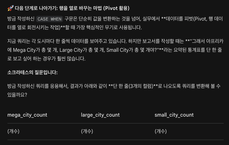
select
    sum(case when c.population >= 5000000 then 1 else 0 end) as 'mega_city_count',
    sum(case when c.population < 5000000 and c.population >= 1000000 then 1 else 0 end) as 'large_city_count',
    sum(case when c.population < 1000000 then 1 else 0 end) as 'small_city_count'
from city c
join country cn
on c.countrycode = cn.code
where cn.continent = 'Africa'
select
count(case when c.population >= 5000000 then 1 end) as 'mega_city_count',
count(case when c.population < 5000000 and c.population >= 1000000 then 1 end) as 'large_city_count',
count(case when c.population < 1000000 then 1 end) as 'small_city_count'
from city c
join country cn
on c.countrycode = cn.code
where cn.continent = 'Africa'- count 함수는 기본적으로 NULL 값을 무시하여 세지 않기 때문에 ELSE 0을 생략해도 동일하게 작동함
- but sum 함수는 NULL 값을 무시하지 않기 때문에 해당 조건이 0개라면 0이 아닌 NULL 값이 리턴됨
- 그룹화 조건을 사용한다면?

select
    cn.continent,
    count(case when c.population >= 5000000 then 1 end) as 'mega_city_count',
    count(case when c.population < 5000000 and c.population >= 1000000 then 1 end) as 'large_city_count',
    count(case when c.population < 1000000 then 1 end) as 'small_city_count'
from city c
join country cn
on c.countrycode = cn.code
group by cn.continent
- 그룹화 결과에 필터링 조건을 추가한다면?

select
    cn.continent,
    count(case when c.population >= 5000000 then 1 end) as 'mega_city_count',
    count(case when c.population < 5000000 and c.population >= 1000000 then 1 end) as 'large_city_count',
    count(case when c.population < 1000000 then 1 end) as 'small_city_count'
from city c
join country cn
on c.countrycode = cn.code
group by cn.continent
having count(case when c.population >= 5000000 then 1 end) >= 1
# having mega_city_count >= 1
[ 텍스트 분석 ]
긍정/부정 고유 키워드 추출
같은 단어가 긍정·부정 양쪽에 모두 등장하면, 감성을 구분하는 데 도움이 되지 않는다. 따라서 각 그룹에만 고유하게 등장하는 키워드를 뽑아야 한다.
TF-IDF 차이 방식
긍정 평균 TF-IDF − 부정 평균 TF-IDF
- 큰 양수 → 긍정 리뷰에서만 자주 등장하는 긍정 고유 키워드
- 큰 음수 → 부정 리뷰에서만 자주 등장하는 부정 고유 키워드
- 0 근처 → 양쪽 모두 비슷하게 쓰이는 공통 단어 (구분력 없음)
코드 흐름
Step 1: 긍정/부정 그룹별 평균 TF-IDF 벡터 계산
pos_mean = tfidf_combined_matrix[pos_indices].mean(axis=0).A1
neg_mean = tfidf_combined_matrix[neg_indices].mean(axis=0).A1
- tfidf_combined_matrix[pos_indices] : 전체 행렬에서 긍정(또는 부정) 리뷰에 해당하는 행들만 추출
- .mean(axis=0) : 열(단어) 방향 평균 → 해당 그룹 내에서 각 단어의 평균 중요도
- .A1 : 2차원 행렬 [[a, b, c, d]]을 1차원 배열 [a, b, c, d]로 평탄화
Step 2: 차이 계산
diff_mean = pos_mean - neg_mean
Step 3: 고유 키워드 상위 추출
# 긍정 고유: 내림차순 정렬 → 양수만
pos_unique_idx = diff_mean.argsort()[::-1]
pos_unique_idx = pos_unique_idx[diff_mean[pos_unique_idx] > 0]

# 부정 고유: 오름차순 정렬 → 음수만
neg_unique_idx = diff_mean.argsort()
neg_unique_idx = neg_unique_idx[diff_mean[neg_unique_idx] < 0]
워드클라우드 시각화
텍스트 데이터에서 단어의 빈도나 중요도를 글자 크기로 시각화하는 방법이다. 빈도가 높을수록 글자가 크게 표시되며, 보고서나 발표 자료에 자주 활용된다.
전체 리뷰 워드클라우드
wc = WordCloud(
    font_path=font_path, width=800, height=400,
    background_color='white', max_words=100, colormap='viridis'
)
wc.generate(all_text)
긍정/부정 고유 키워드 워드클라우드
- generate_from_frequencies(dict) : 빈도 딕셔너리를 기반으로 워드클라우드 생성
- 긍정은 Greens, 부정은 Reds 컬러맵 사용
마스크 이미지를 활용한 워드클라우드
from PIL import Image
pos_mask = np.array(Image.open('images/mask_heart.png').convert('L'))
- .convert('L') : 이미지를 흑백 1채널로 변환 (가로×세로 픽셀마다 1개의 값)
- mask 파라미터에 넘기면 해당 모양 안에만 단어가 배치됨
하나의 워드클라우드에 긍정/부정 색상 구분하기
recolor(color_func=...) 를 사용하면 단어별로 색상을 직접 지정할 수 있다.
def sentiment_color(word, **kwargs):
    if word in positive_words:
        return "#2E8B57"   # 초록 (긍정)
    elif word in negative_words:
        return "#DC143C"   # 빨강 (부정)
    else:
        return "#999999"   # 회색 (중립)

wc_combined.recolor(color_func=sentiment_color)
- 범례는 matplotlib.patches.Patch로 추가
별점별 키워드 변화 추적
별점 1점과 3점은 같은 '부정'이지만 불만의 정도가 다르다. 이분법(긍정/부정) 대신 별점 1~5 각각의 키워드가 어떻게 달라지는지 세밀하게 추적한다.
별점 예상 특징
| 1점 | 강한 불만, 결함, 반품/환불 |
| 2점 | 기대 이하, 부분적 불만 |
| 3점 | 보통, 장단점 혼재 |
| 4점 | 대체로 만족, 사소한 아쉬움 |
| 5점 | 강한 만족, 재구매/추천 |
별점별 TF-IDF 키워드 추출
for rating in sorted(df_sample['rating'].unique()):
    rating_idx = df_sample[df_sample['rating']==rating].index.to_list()
    keywords = get_top_tfidf_keywords(tfidf_combined_matrix,
                                     combined_feature_names, rating_idx, top_n=10)
    rating_keywords[rating] = keywords
히트맵 시각화
sns.heatmap()으로 별점(행) × 키워드(열)의 TF-IDF 평균 값을 색상 강도로 표현하면, 별점에 따른 키워드 중요도 변화를 한눈에 파악할 수 있다.
동시출현(Co-occurrence) 분석
N-gram은 바로 옆에 붙어 있는 단어 조합만 포착한다. 반면 동시출현 분석은 같은 문서(리뷰) 안에 함께 등장하는 단어 관계를 포착한다.
N-gram 동시출현
| 조건 | 단어가 바로 옆에 연속 등장 | 같은 문서 안에 함께 등장 |
| 예시 | "어깨 통증" (붙어야 함) | "어깨…편하다" (떨어져도 OK) |
| 포착 | 구문(phrase) 패턴 | 개념 간 관계(association) |
| 시각화 | 막대 그래프 | 네트워크 그래프 |
동시출현 행렬 만드는 법
co_vec = CountVectorizer(ngram_range=(1,1), max_df=0.85, min_df=3, binary=True)
co_dtm = co_vec.fit_transform(df_sample['processed'])

co_matrix = co_dtm.T @ co_dtm   # 단어 × 단어 동시출현 행렬
co_matrix.setdiag(0)             # 대각선(자기 자신) 0으로
- binary=True : 한 리뷰에서 단어가 여러 번 반복되어도 1로만 기록 → DTM.T @ DTM의 결과가 정확히 두 단어가 함께 등장한 리뷰 수가 됨
- 대각선 제거 : 자기 자신과의 동시출현은 의미 없으므로 0으로 설정
상위 동시출현 쌍 추출
co_pairs = []
for i in range(len(co_words)):
    for j in range(i + 1, len(co_words)):  # 상삼각만 순회 → 중복 방지
        if co_array[i, j] > 0:
            co_pairs.append((co_words[i], co_words[j], co_array[i, j]))
co_pairs.sort(key=lambda x: x[2], reverse=True)
네트워크 시각화
pyvis 라이브러리의 Network를 사용하여 인터랙티브 네트워크 그래프(HTML)를 생성한다.
- 노드 크기 : 연결된 간선 가중치 합으로 min-max 정규화
- 간선 두께 : 동시출현 횟수에 비례
- 긍정/부정 각각의 서브 DTM으로 별도 네트워크 생성 가능
정리 및 핵심 요약
- 텍스트 전처리 파이프라인 5단계 : 정제 → 정규화 → 형태소 분석 → 불용어 제거 → 공백 Join
- N-gram으로 단어 조합 패턴 포착 : Unigram(개별 단어), Bigram(연속 2단어)
- TF-IDF로 각 그룹의 핵심 키워드 추출 : TF(문서 내 빈도) × IDF(역문서 빈도) → 특정 문서에서 진짜 중요한 단어
- min_df/max_df 필터링 : max_df=0.85(공통 단어 자동 제거), min_df=3(희귀 단어 제거)
- 워드클라우드 : 전체·긍정/부정 고유·마스크·통합 색상 구분 워드클라우드
- 별점별 키워드 변화 추적 : 히트맵으로 별점에 따른 키워드 중요도 변화 시각화
- 동시출현 분석 : DTM.T @ DTM으로 동시출현 행렬 생성 → 네트워크 그래프로 단어 간 연결 관계 시각화
추가: 영어 빈도 분석
영어의 "형태소 분석"은 토큰화 + 표제어 추출(Lemmatization) 이다.
- 한국어: "먹었습니다" → Kiwi → ['먹', '었', '습니다']
- 영어: "cars running" → NLTK → ['car', 'run']
설치 및 데이터 다운로드
# 터미널
uv add nltk

# 코드 내 최초 1회
import nltk
nltk.download('punkt')
nltk.download('punkt_tab')
nltk.download('wordnet')
nltk.download('averaged_perceptron_tagger')
토큰화 + 표제어 추출
from nltk.tokenize import word_tokenize
from nltk.stem import WordNetLemmatizer

lemmatizer = WordNetLemmatizer()

def extract_english_tokens(text):
    tokens = word_tokenize(text.lower())                          # 소문자 변환 + 토큰화
    lemmas = [lemmatizer.lemmatize(token) for token in tokens]    # 표제어 추출
    return [w for w in lemmas if w.isalpha() and len(w) >= 2]     # 알파벳만, 2글자 이상
영어 불용어 제거
한국어에서는 불용어 리스트를 직접 만들어 제거했지만, 영어에서는 TfidfVectorizer(stop_words='english')로 자동 처리할 수 있다.
from sklearn.feature_extraction.text import TfidfVectorizer
from sklearn.feature_extraction._stop_words import ENGLISH_STOP_WORDS

domain_stopwords = {'inc', 'llc', 'corp', 'company', 'co'}
combined_stopwords = list(ENGLISH_STOP_WORDS | domain_stopwords)

tfidf = TfidfVectorizer(
    stop_words=combined_stopwords,
    max_df=0.85,
    min_df=3,
    max_features=3000
)
MPS란?
MPS는 Apple 기기에 탑재된 물리적인 GPU를 활용하여 고성능 연산(딥러닝, 이미지 처리 등)을 수행할 수 있도록 도와주는 소프트웨어 프레임워크(API)이다.
- 하드웨어: Mac에 내장된 그래픽 연산 장치 (Apple Silicon GPU)
- 소프트웨어(MPS): PyTorch가 내리는 수학적 명령(행렬 곱셈 등)을 Apple GPU가 알아듣고 최대한 빠르게 계산하도록 번역하고 최적화해 주는 엔진
import torch

# MPS를 통한 GPU 가속이 현재 OS와 하드웨어에서 지원되는지 확인
is_mps_available = torch.backends.mps.is_available()
print(f"MPS 사용 가능 여부: {is_mps_available}")

if is_mps_available:
    device = torch.device("mps")
    print("Apple GPU(MPS)를 연산 장치로 사용합니다.")
else:
    device = torch.device("cpu")
    print("MPS를 지원하지 않아 CPU를 사용합니다.")
1. BERT 모델 개요
TF-IDF는 단어의 문맥을 이해하지 못한다는 한계가 있다.
문장 TF-IDF가 보는 것 실제 의미
| "이 영화 재미없다" | "재미" => 긍정? | 부정! |
| "이 영화 재미있다" | "재미" => 긍정? | 긍정! |
| "연기가 좋지 않다" | "좋" => 긍정? | 부정! |
→ TF-IDF는 개별 단어만 보기 때문에 부정 표현, 문맥 의존적 의미를 놓친다.
그래서 등장한 BERT!
BERT는 텍스트의 문맥을 양방향으로 이해한다.
- 사전학습(Pre-training) : 위키피디아 등 대규모 텍스트로 언어의 일반적인 패턴을 미리 학습
- 파인튜닝(Fine-tuning) : 감성 분류 등 특정 과제에 맞게 추가 학습
- 양방향 문맥 이해 : 단어의 왼쪽과 오른쪽 문맥을 동시에 고려
Hugging Face
AI 모델을 공유하고 사용할 수 있는 오픈소스 플랫폼이다. 개발자들이 GitHub에서 코드를 공유하듯, AI 연구자들은 Hugging Face에서 학습된 모델을 공유한다.
Pipeline이란?
Hugging Face의 pipeline()은 모델 + 토크나이저를 한 줄로 사용할 수 있게 해주는 편리한 도구이다.
# 이 한 줄이 내부적으로 수행하는 작업:
classifier = pipeline("sentiment-analysis")

# 1. 토크나이저 로드 => 텍스트를 숫자(토큰)로 변환
# 2. 모델 로드 => 토큰을 입력받아 예측 수행
# 3. 후처리 => 예측 결과를 사람이 읽기 쉬운 형태로 변환
실습에서 사용하는 방법
from transformers import pipeline
classifier = pipeline("sentiment-analysis", model="모델이름")

# 사용 예시
result = classifier("이 영화 정말 재밌어요!")
# => [{'label': '1', 'score': 0.9875}]  (1=긍정, 0=부정)
모델 찾는 방법
- https://huggingface.co/models 에 접속
- Task 필터에서 Text Classification 선택
- Language 필터에서 데이터셋에 맞는 언어 (예: Korean) 선택
- 원하는 세부 작업을 검색창에 입력 (예: 감성 분석이면 sentiment, 스팸 분류면 spam)
- 후보 모델의 모델 카드에서 평가 지표(Accuracy, F1 등) 확인
- 다운로드 수, 좋아요 수도 함께 참고하여 검증된 모델을 선택
Hugging Face 덕분에 대규모 AI 모델을 직접 학습하지 않아도, 이미 학습된 모델을 pipeline() 한 줄로 바로 사용할 수 있다.
'[데이터분석] 부트캠프 TIL' 카테고리의 다른 글
| 20260317 TIL (0) | 2026.03.17 |
|---|---|
| 20260316 TIL (1) | 2026.03.16 |
| 20260312 TIL (0) | 2026.03.12 |
| 20260311 TIL (0) | 2026.03.11 |
| 20260305 TIL (0) | 2026.03.05 |